
SimOne Version History
SimOne 2.7 Changelog
Changes in Version 2.7
What’s new in SimOne 2.7
SimOne Updater
The SimOne Updater works if the internet connection is active. It provides a fast and easy way to update the SimOne version to the latest published one. When updated the reserve copy of the current version is performed and the user can later roll back to it.
The Updater window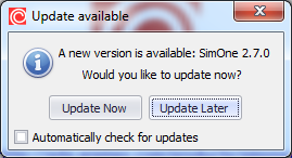
is called with the Check for new version button at the About SimOne window (Help → About SimOne… menu entry).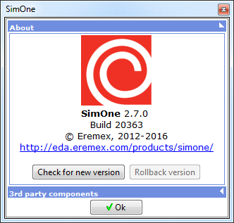
The Rollback to the previous version is made with the corresponding button.
Math expressions
New functions for Fourier transform are added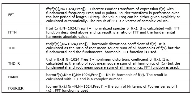
These functions can be used in expressions to be plotted at graphs, but cannot be used in expressions describing components behavior.
An example of using the Fourier transforms is shown in fft_based_func.sschfile contained in FFT folder of SimOne examples. It can be opened with File→Examples… menu entry.
Fixes
- Some known issues with subcircuits are fixed.
SimOne 2.6 Beta Changelog
Changes in Version 2.6 Beta
New Features in SimOneUser FeedbackThe feedback with a message to the developers can now be sent from inside SimOne. With the Help→Feedback menu entry “Contact developer” window is opened.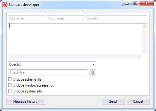
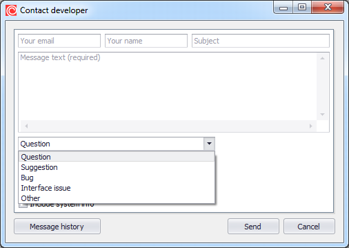
At the window there are optional fields for the sender email, name and the message subject. The message text cannot be left blanc. If the message type is Question, the email to send the response must be provided too.
The message types are:
- Question,
- Suggestion,
- Bug,
- Interface issue
- or Other.
Additional information can be send:
- Scheme (or netlist),
- Current SimOne view screenshot (without Contact developer window),
- System information,
-Any other file.
The sent messages are stored in the history. To view them click the Message history button.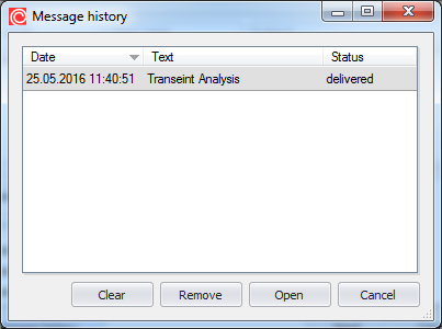
Touchstone model and N-port devices
SimOne now supports N-port components, specified with S-, Z- and Y-parameters.
The parameters can be set either as expressions or as Touchstone files.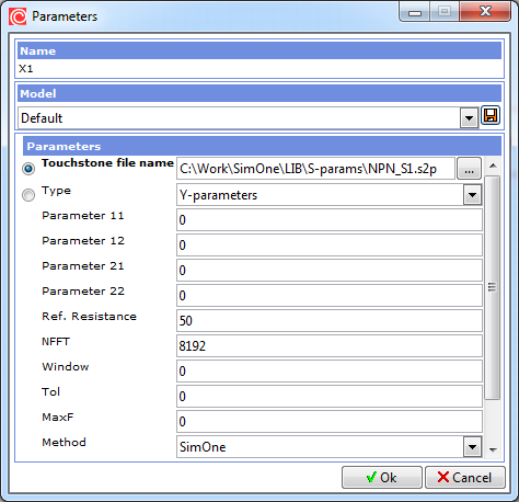
N-ports can be placed to the schematic eitheras a primitive (toolbar icons ![]() ) ora component from included libraries of Touchstone-models:
) ora component from included libraries of Touchstone-models: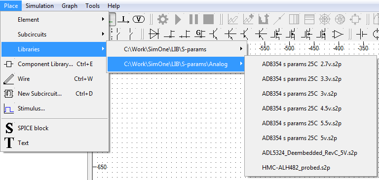
A new property is introduced for Laplace sources and N-ports: MaxF. It defines the Inverse Fourier Transform step applied to the specified element (or model) in simulations. Note: this doesn't define the element itself, but only the behaviour of computational algorithms.
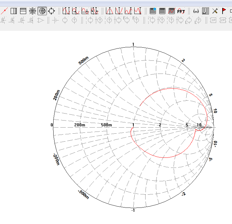
Graphs
Graphs in AC analysis can be displayed on the Smith chart.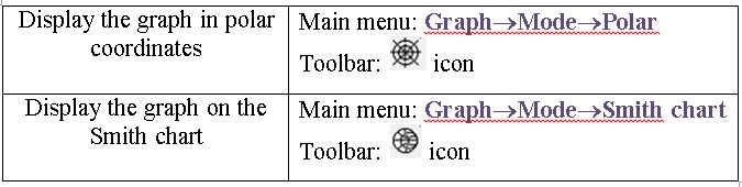
Export
AC analysis graphs can be exported in Touchstone and Freq formats.
Export to a Touchstone-file window: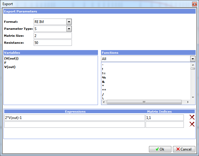
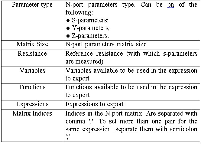
It contains the following parameters: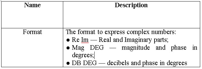
Export to a Freq-file window: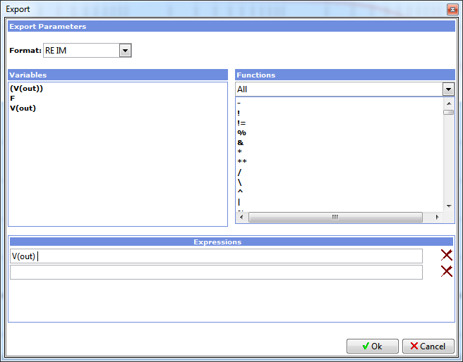
Рис. 20.16.5 Окно экспорта графика в Freq-файл
It contains the following parameters: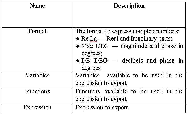
Mathematical expressions
The following measurements can now be used as expressions: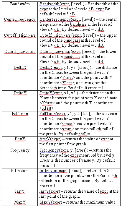
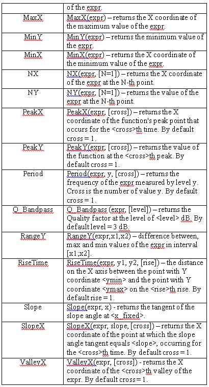
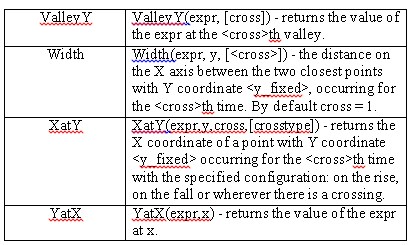
However, they can be used in expressions to plot as graphs, but not in descriptions of schematic components.
Fixes
Metric suffixes interpretation errors are fixed.
SimOne 2.5 Changelog
Changes in Version 2.5
Laplace sources
- Functional voltage and current sources, defined with Laplace transfer function are now moved to a separate component group in the Schematic. Each Laplace source has its own graphical symbol.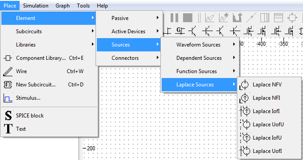
- New algorithms for convolution integral computation in Laplace sources have been added. Previously used algorithms get more manually chosen parameters.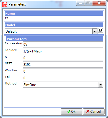
ParameterDescriptionDefault valueUnitLaplaceLaplace transfer function1/(s + 1Meg) RInner resistance0OhmNFFTNumber of points used for Inverse Fourier Transform8192—WindowThe interval of non-zero values of the transfer function in time-domainTendsecTolMinimal absolulte value of the function in the convolution integral0—Method Numerical method for computation of Inverse Laplace Transform and the convolution integral. Three methods are available:
- SimOne — the original method
- IFT — Inverse Fourier Transform usage for ILT and trapezoidal rule for the convolution integral
- Euler — Fourier-series method with Euler summation for ILT and and trapezoidal rule for the convolution integral SimOne - The transfer function can be given as a table of values. The special functions with “freq_” prefix are used for this.
Periodic Steady-State
Periodic Steady-State analysis has a new interface.
- Time interval for plotting the graphs is now set in number of periods. The default value is 10.
- The maximal time step is set with minimal number of steps per period, the default value of which is 20.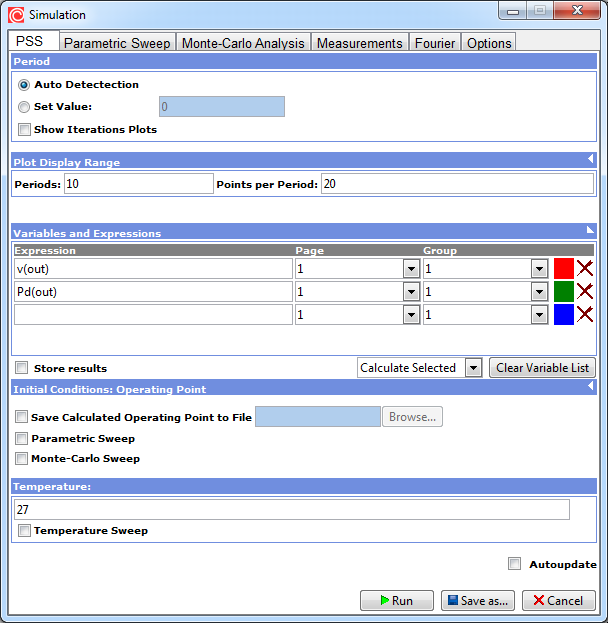
Piecewise Linear input signals
New parameters for Piecewise Linear (PWL) signals are available:
ParameterDescriptionDefault valuePWL_Method PWL processing method
- Standard SPICE method
- SIMONE: tries to consider the PWL signal as points of some smooth signal SIMONEPWL_BPRELTOLRelative tolerance for SIMONE method comparison of PWL slopes1PWL_BPABSTOLAbsolute tolerance for SIMONE method comparison of PWL slopes1e-6
Graphs
- Graphs axes can be switched between Linear/Logarithmic scales
X axis in logarithmic scale Main menu: Graph → Log X
Icon: ![]() Y axis in logarithmic scale Main menu: Graph → Log X
Y axis in logarithmic scale Main menu: Graph → Log X
Icon: ![]()
- It is possible to choose the view area of graphs manulally:
Set the view borders for a group of traces Main menu: Graph → View rectangle…
Icon:
- Grpahs can be imported from SimOne simulation data files.
Mathematical expressions
New functions for integral transforms are added:
laplacelaplace(f(x), H(s)) — the convolution of f(x) with the transfer function H(s) given in s-domain. Uses SimOne method.laplace_smnlaplace_smn(f(x), H(s)) — same as laplace.laplace_eulerlaplace_euler(f(x), H(s), mtol) — the convolution of f(x) with the transfer function H(s) given in s-domain. Uses Fourier-series method with Euler summation. Values f(x) < mtol are ignored.laplace_iftlaplace_ift(f(x), H(s), window, nfft, mtol) — the convolution of f(x) with the transfer function H(s) given in s-domain. Uses Inverse Fourier Transform. If window is specified, the frequency step is 0.5/window. The number of values used for IFT is equal to nfft. Values f(x) < mtol are ignored.freq_dbfreq_db(f(x), w1, db1, deg1, …, wn, dbn, degn) — the convolution of f(x) with the transfer function given in frequency-domain with discrete points as [frequency w, magnitude in decibels; argument in degrees] triples.freq_db_degfreq_db_deg(f(x), w1, db1, deg1, …, wn, dbn, degn) — same as freq_db.freq_db_radfreq_db_deg(f(x), w1, db1, rad1, …, wn, dbn, radn) — the convolution of f(x) with the transfer function given in frequency-domain with discrete points as [frequency w, magnitude in decibels; argument in radians] triplesfreq_mafreq_ma(f(x), w1, amp1, deg1, …, wn, ampn, degn) — the convolution of f(x) with the transfer function given in frequency-domain with discrete points as [frequency w, magnitude in absolute values; argument in degrees] triples.freq_ma_degfreq_ma_deg(f(x), w1, amp1, deg1, …, wn, ampn, degn) — same as freq_ma.freq_ma_radfreq_ma_rad(f(x), w1, amp1, rad1, …, wn, ampn, radn) — the convolution of f(x) with the transfer function given in frequency-domain with discrete points as [frequency w, magnitude in absolute values; argument in radians] triples.freq_rifreq_ma_rad(f(x), w1, re1, im1, …, wn, ren, imn) — the convolution of f(x) with the transfer function given in frequency-domain with discrete points as [frequency w, real part, imaginary part] triples.
Bug fixes
- Laplace function in AC analysis is fixed
- Etc.
SimOne 2.4 Changelog
Changes in Version 2.4
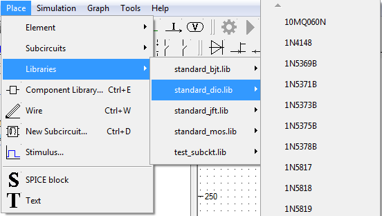
External libraries support
All included external libraries — SPICE-libraries and SimOne schematic-files containing subcircuits — are now shown in “Place” menu. Any component of the libraries is available for placing to the schematic.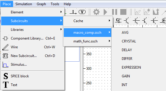
Events
SimOne can track different events happening during circuit simulations, namely
- Local minimum of an expression is found,
- Local maximum of an expression is found,
- Certain value of an expression is reached (optional: from a specified side),
- Certain value of a curve slope is reached (optional: from a specified side),
- Inflection point is found,
- Any specified condition (IF expression) is satisfied.
An event can be set to take one of the following actions as it happens:
- Pause simulation,
- Stop simulation,
Just write the event time into the Log.
Event window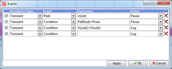
Statistical analysis in Multi-variant analyses
Monte-Carlo analysis/Worst case analysis is added to multi-variant analyses. It allows analyzing the circuit with one or more its parameters distributed in some range. For any parameter of a single element, component model or signal source or a global parameter the distribution range and law can be set.
The statistical analysis runs multiple simulations with different values of the chosen parameters. As a result of the analysis families of desired graphs and histograms of studied characteristics are presented.
SPICE-format
.MC < expression1> … …
Examples
.MC 100 tran V(out) I(Rн) Vmax Imax
.MC 10 ac db(V(Rн)) Band1
.MC 100 dc I(Rн) Imax
Monte-Carlo Analysis tab of the Simulation window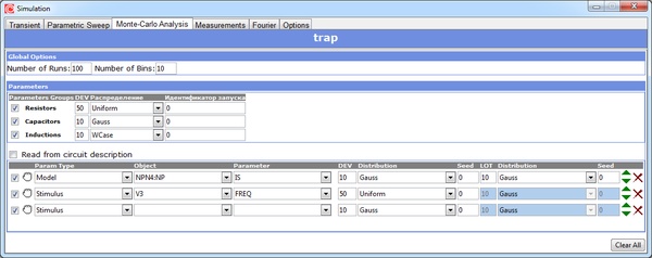
Histograms
Histograms are an alternative way of presenting simulation results and show the numerical values of plots distribution by chosen intervals.
Add Histogram window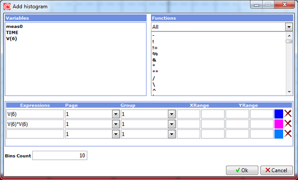
Histogram view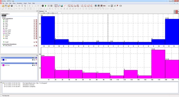
.WAV-files
Signals can now be set in the form of sound (as .wav-files). Plots as well can be exported as .wav-files and played directly in SimOne.
Mathematical expressions
- Random value generators with different distributions, and Integral transforms are added.
Fixes
- Bug with PWL-signals
- Etc.
SimOne 2.3 Changelog
Changes in Version 2.3
What’s new in SimOne 2.3
Monte-Carlo / Worst Case Analysis
Monte-Carlo analysis performs multiple runs of a certain type of analysis (e.g. Transient) with different values of specified parameters (of elements, component models, stimuli or global parameters). For each run the values are randomly chosen within the user-specified ranges according to selected probability distributions. Performance characteristics are calculated and presented graphically as histograms. A set of graphical plots corresponding to the chosen analysis type.
Monte-Carlo parameters window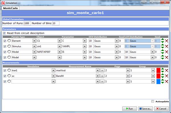
Performance characteristic hystogram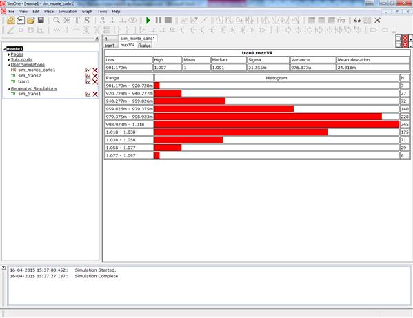
For the Worst Case analysis the WCase and AWCase distributions are chosen. In this case for each run only the border values of the parameter are selected.
Sensitivity Analysis
Sensitivity analysis is used for determining what influence parameters of circuit components have on one or more output expressions. Sensitivity analysis is usually performed before the circuit optimisation, since it helps to choose among the parameters to be varied, thus increasing the speed and effectiveness of the optimisation. As well it helps to find the parameters, which have the most influence on performance characteristics, the results being used in Monte-Carlo/Worst Case.
Sensitivity analysis parameters window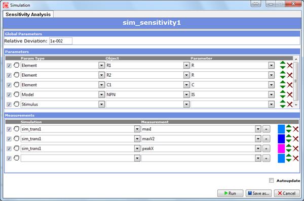
The sensitivity analysis results for each measurement are presented in an individual tab. In the table the absolute and normalised sensitivities are given. The histogram for the chosen sensitivity (absolute or normalised) is displayed. It can be switched with the corresponding button.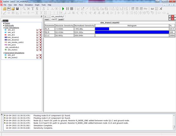
DC Sensitivity Analysis
DC Sensitivity analysis estimates the influence of circuit components, model parameters or temperature on DC output expressions in order to determine the most important variables.
SPICE syntax:
.SENS ...
is the output expression to estimate the sensitivity
Examples:
.SENS v(out)
.SENS {v(out)*I(Rout)} Vbe(Q1)
DC Sensitivity analysis parameters window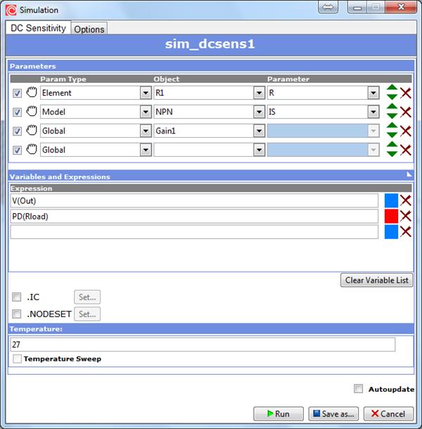
The sensitivity analysis results for each output expression are presented in an individual tab. In the table the absolute and normalised sensitivities are given. The histogram for the chosen sensitivity (absolute or normalised) is displayed. It can be switched with the corresponding button.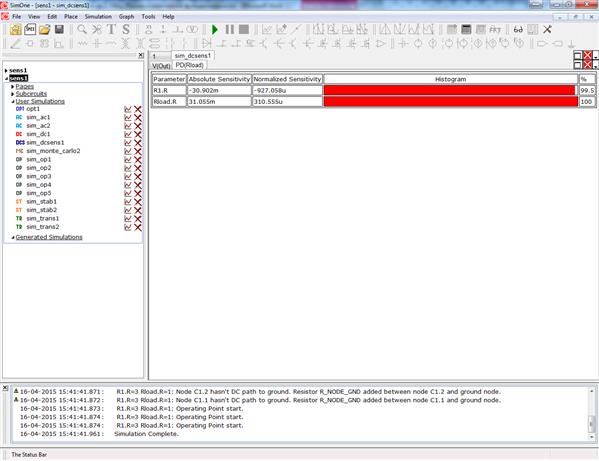
Fourier Transform
Fourier Transform can be now specified with:
SPICE-command .FOUR;Fourier tab in Simulation parameters windows;Fourier Transform window during the post-processing.
.FOUR command can be written down if a SPICE-netlist is used or in a SPICE-text block in the Schematic editor.
SPICE/LTSPICE syntax:
.FOUR [] []
+ ...
Examples:
.four 1KHz V(out)
.four 10KHz 3 V3(out)
Fourier Transform tab is available on the following analyses windows:
- Transient analysis
- Periodic Steady-State analysis
- AC analysis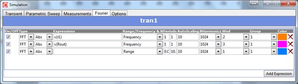
Fixes
- Operational amplifier model
- Various minor bugs
SimOne 2.2.1 Changelog
Changes in Version 2.2.1
What’s new in SimOne 2.2.1
- The special variables ’f’ and ’hertz’ are now available in AC analysis, reflecting the frequency. In other analysis ’f’ and ’hertz’ are zero.
Example:
E1 1 0 value={hertz*v(1)+f^2*i(v1)}
- TABLE and PWL functions are now allow to set their parameters from txt file:
wl(Expression,«File name»), table(Expression,«File name»).
Example:
pwl(v(1),«Curve1.txt»), table(sin(v(1))*i(v1)," Curve1.txt»).
Curve1.txt:
0 0
0.1 10
0.3 60
1.0 1e3
- The gain of the Opamp now can be set via Expression.
Fixed
- Component base objects proceeding in Schematic.
- Etc.
SimOne 2.2 Changelog
Changes in Version 2.2
Schematic
- Text component for SPICE definitions of the circuit has been added. It can be used for defining the circuit or its parts, including files that contain models or defining new models, setting simulation commands, postprocessing commands and any other valid SPICE commands that can be included into a SPICE netlist.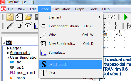
- circuit storage files format has been changed;
- interface of text components of the editor is improved.
Measurements
- .meas[ure] command for Measurements is now supported in HSPICE/LTSPICE/NGSPICE formats;
- Measurement command in SimOne format is added.
Example:
Signal period finding
HSPICE/LTSPICE:
.meas period trig v(out)=0.5 rise=6 targ v(out)=0.5 rise=7
SimOne:
.meas period1 period v(out) 0.5 11
Bandpass width finding:
HSPICE/LTSPICE:
.meas ac tmp max mag(V(out))
.meas ac Bandwidth trig mag(V(out))=tmp/sqrt(2) rise=1
+ targ mag(V(out))=tmp/sqrt(2) fall=last
SimOne:
.meas ac Band1 Bandwidth mag(v(out))
SPICE-netlist translator
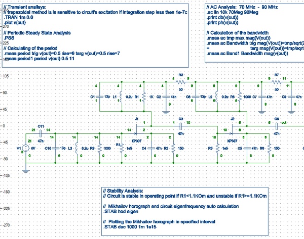
- Circuit stability analysis command:
.stab hod [log/lin] [eigen] — automatic stability computation
hod — use Mikhailov hodograph;
log/lin — hodograph plotting options;
eigen — circuit eigenvalues computation.
.stab lin/dec/oct < stop> — hodograph plotting in the given interval
— step or points number within the interval;
, — left and right borders of the interval.
- Periodic Steady State calculation command:
.pss [] [] [] []
— the period of the process, automatically determined if not set;
— stabilization periods number;
— maximal iterations number;
— accuracy tolerance.
- Etc.
Simulation
- Convergence of the dc sweep analysis is improved;
- Kirchhoff currents law control is corrected;
- Simulations management is improved.
Mathematical expressions
- Integer division quotient — \ or DIV — and remainder — % or MOD — operators has been added.
Bug-fixes in
- .IC command and UIC option in Transient analysis;
- etc.
SimOne 2.1 Changelog
Changes in Version 2.1
Components
The following components models have been introduced:
— Dependent sources described with a Laplace Transmission Function
SPICE-description:
E1 2 0 1 0 Laplace = s/(2*s^2+s*2+1) – voltage source
G2 4 0 1 0 Laplace = exp(-s) – current source
Schematic: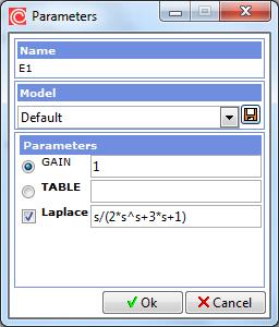
— Functional sources described with a Laplace Transmission Function
SPICE-description:
E2 2 0 LAPLACE{V(1)+V(1)*V(2)} = s/(2*s^2+3*s+1) – voltage source
B2 2 0 V = {V(1)+V(1)*V(2)} laplace = {s/(2*s^2+3*s+1)} – voltage source
G2 3 0 LAPLACE{V(1)+V(1)*V(2) } = exp(-s) – current source
B3 3 0 I = {V(1)+V(1)*V(2)} laplace = {exp(-s)} – current source
Schematic: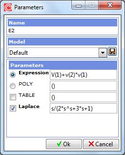
— Independent sources described with an arbitrary ‘Expression’
SPICE-description:
E2 2 0 Value = {stp(2)*sin(t)} – voltage source
B2 2 0 V = {stp(2)*sin(t)} – voltage source
G2 3 0 Value = {stp(2)*sin(t)} – current source
B3 3 0 I = {stp(2)*sin(t)} – current source
Schematic: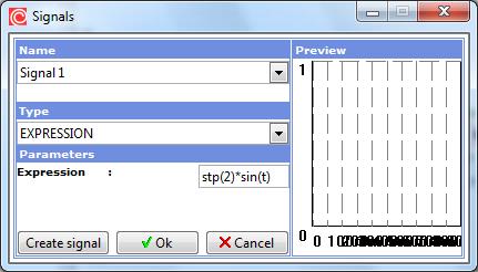
Simulation
— Transient methods convergence is significantly improved;
— Kirchhoff's circuit laws observance is improved;
— Development processes interactivity is widened: simulations can be automatically recalculated when editing Schematics or SPICE-netlists;
— New block methods for matrices are added. Large matrices decomposition is made quicker with them and the simulation speed is significantly increased. Simulation of large circuits is now tens and hundreds times faster.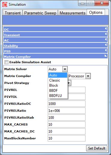
The matrix compiler ‘MatrixSolver’ property default value corresponds to the automatic choosing of a decomposition algorithm depending on the circuit dimension.
Mathematical expressions
— Mathematical constants PI = 3.14159265358979323846 and E = 2.71828182845904523536 are now recognized;
— Complex numbers can be used with I, i, J or jas a square root of -1: 1+I, 1+i, 1+J, 1+j.
Functions
Impulse(X) — Impulse function of amplitude X and area 1;
STP(X), U(X) — Step function of amplitude 1.0 starting at T >= X;
uramp(X) — X*U(X);
DDT(x), SDT(x), IDT(x), IDTMOD(x) — numerical differentiation and integration;
EXPL(x, max) — exponential function with linear continuation: EXPL(x, max) = exp(x) for x <= max and EXPL(x, max) = exp(max)*(x + 1 – max) otherwise;
BUF(x) — 1 for x > 0.5, otherwise 0;
inv(x) — 0 for x > 0.5, otherwise 1;
ceil(x), floor(x) — rounding to up or down to the closest integer.
SPICE-netlist translator
— SPICE file parsing speed is significantly increased;
— .define and .include directives support is added;
— Arbitrary voltage and current sources can now be included as B-components: B1 1 0 V = {uramp(2)*sin(t)} etc.;
— SPICE-libraries (.lib) using is corrected.
Schematic
— Global parameters in the Schematic are now supported: the window for setting circuitwise global SPICE-directives (.param, .define, .func) is now available.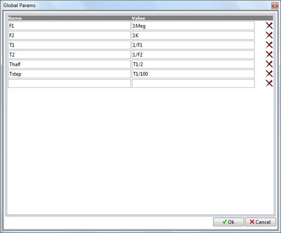
— The interface for working with the Schematic text components is improved.
Bug-fixes in
— AC Point simulation results display;
— NODESET command;
— etc.
SimOne 2.0.2 Beta Changelog
Changes in Version 2.0.2 Beta
What’s new in SimOne 2.0.2
- A dot-separator for subcircuit components is added, example X1.R1,X1:R1, X2.X1.Q2, X2:X1:Q2
Fixed:
- PSS Analisys for circuits without inductors and capacitors;
- Signals of the subcircuits;
- Time variable in expressions inside component models;
- etc.
SimOne 2.0.1 Beta Changelog
Changes in Version 2.0.1 Beta
What’s new in SimOne 2.0.1 Beta
- the functions of the numerical integration sdt() and differentiation ddt() are added for transient analysis;
- the initial point is added for sd(),avg(),rms() functions.
Fixed:
- Win XP/Vista compatibility;
- opamp models in component base;
- transmission line model;
- transient analysis bugs;
- etc.
SimOne 2.0 Changelog
Changes in Version 2.0 Beta
SimOne 2.0. What’s new?
Circuit Optimizer
Parametric optimizer in SimOne provides automatic circuit tuning by searching for such values of components parameters that give desired values of certain circuit properties.
One can tune parameters of single components or of component models, parameters of source signals and global parameters as well.
There are two ways of setting a function to be optimized:
Using Measurement Tools for simulation results. It can either be a demand on a certain measurement to be maximized/minimized/kept in constraints;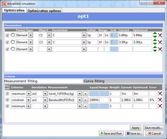
Specifying a graphical curve — a desired behavior of the circuit’s output parameters. The deviation of the real curve from the desired one is minimized then.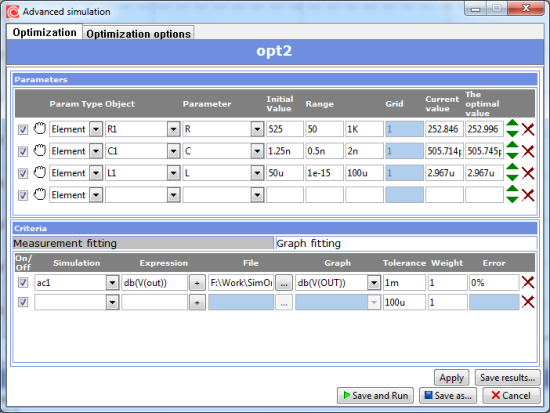
Several methods of optimization are available: Powell’s method, Nelder–Mead method or Differential evolution.
Optimization results can be saved into a text file (![]()
![]() ). Current parameters of circuit components can be replaced with the optimal ones with button.
). Current parameters of circuit components can be replaced with the optimal ones with button.
Optimization task is set with Simulation → Optimization... menu entry.
Circuit components parameters tuning
It is possible now to make a manual circuit tuning in SimOne. Manual tuning is an interactive process of varying certain parameters with manipulating the correspondent sliders. That causes automatic recalculation of circuit characteristics and the desired behavior can be found.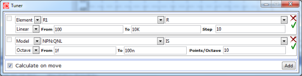
The same parameters can be varied as for Optimization: parameters of single components, of component models, of source signals and global parameters.
Ways of varying are standard: linearly, by octaves, by decades and by a given list.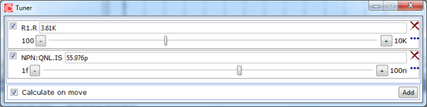
Parameter tuning is called with Simulation → Tune Parameters… menu entry.
Viewing current values of component parameters
Each circuit component has its own data list that can be viewed. It includes all input parameters of the component model and some output as well, such as current, power, capacity, charge etc.
All those parameters, nodes voltages and any mathematical expressions of them can be viewed in the Watch window (View → Watch).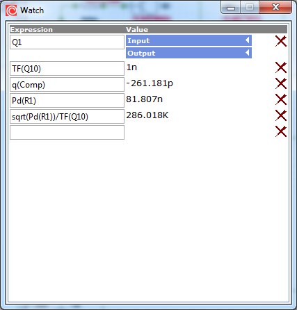
The current state of the circuit can be saved in a text file with Simulation → State output. Current state of all components and state variables is presented there.
Components
The following non-linear components are now added:
Non-linear resistors,Non-linear capacitors,Non-linear inductors. Resistor’s Resistance, capacitor’s Capacitance and Charge, inductor’s Inductance and Flux can now be any mathematical expression of nodes voltages, voltage drops and currents through sources and inductors.
Exporting plots
Plots can now be exported in a plain text format.
SimOne 1.6 Changelog
Changes in Version 1.6
Operating Point Analysis
The Operating Point Analysis is now an interactive process. User can modify the circuit and the current operating point will be recalculated automatically. The results will be shown in a table and displayed at the schematic as well.
Operating Point Analysis window: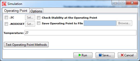
The table of results: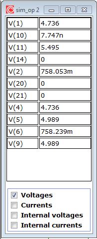
AC Point Analysis
AC Point Analysis calculates the AC voltages and currents and component small-signal parameters at the user specified frequency. AC Point Analysis is an interactive process like the Operating Point Analysis.
AC Point Analysis window: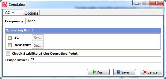
The table of results: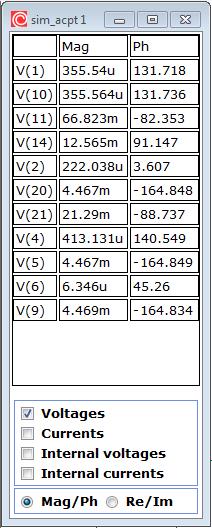
Parametric Sweep
The following parameters can now be stepped:
component attribute parameters;
model parameters;
global parameters(those created with a .DEFINE, .PARAM statement)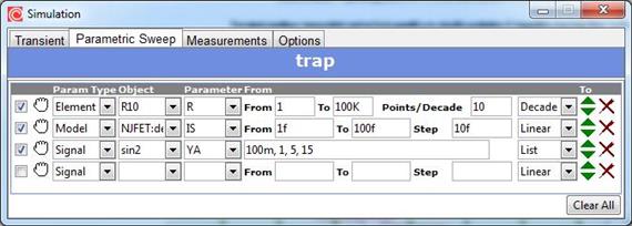
SPICE netlist
The following SPICE commands are now supported:
.IC, .NODESET – for operating point calculation,
.OPTIONS, .OP, .TRAN, .AC, .STEP, .TEMP – for simulations,
.PLOT, .PRINT, .PROBE – for displaying results;Export Schematic to SPICE netlist is now available
SimOne 1.5 Changelog
Changes in Version 1.5.2
What’s new in SimOne 1.5.2
– The Imelt options is added to rule the pn junction currents .
– The special Operating Point Window with .IC and .NODESET commands is added in DC Analysis.
– The sgn(x) ( signum(x) ) function is now supported
Fixed
– Errors in V-SWITCH, I-SWITCH and MOSFET Level =1..3 models
– Etc.
Changes in Version 1.5.1
What’s new in SimOne 1.54.1
The following options in time step control algorithm in Transient Analysis are added:
– LTERELTOL – Relative current tolerance for truncation error;
– LTEABSTOL – Absolute current tolerance for truncation error;
– TRINIT – Initial transient step multiplier: hinit = TRINIT*hmax;
– TRMIN – Minimal transient step multiplier: hmin = TRIMIN*hinit;
Fixed
– Bugs in Transient Analysis and Periodic Steady-State Analysis
– Etc.
SimOne 1.4 Beta Changelog
Changes in Version 1.4.1
What’s new in SimOne 1.4.1 Beta
– Improved operating point calculation algorithms.
– Non-linear components models parameters evaluation is improved.
– Improved SPICE-netlist Editor.
– Improved Capture: wires are easier to connect now.
– Global Component base search is now available.
Fixed
– SPICE-reader bugs
– Errors in Diode, PNP and MOSFET models
– Etc.
Changes in Version 1.4.0
Warning!
It is strongly recommended to set preferences to default when updating your SimOne version for all interface changes to be applied automatically (“Reset to default” button on Preferences window).
SimulationResultsProcessing
— Fourier Analysis.Transient graphs spectre calculation and display based on Fast-Fourier Transform are added.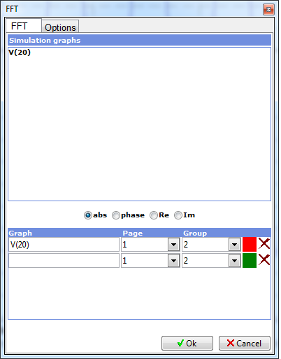
— Measurements in Parametric Sweep analysis are now calculated for each parameter value.
Cursors
New features in using cursors are now available:
— Cursors placement to a certain Measurement result.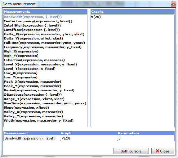
— Cursors placement to certain X and Y values.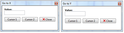
— Fast cursor placement to a graph Peaks, Valleys, Highest and Lowest points (see buttons described below).
Simulation
— Convergence of operation point calculation is improved.
— The control of KCL precision is added for operation point calculation.
— Parametric Sweep interface is improved.
— Measurements tab is added to the Simulation window, so they can be set with other simulation parameters.
— Simulation warnings preferences are added to the Simulation window.
Graph Viewer
— In AC analysis you can switch between Real and Complex plots.
— Buttons for FFT window, cursor functions (see above) are added.
Schematic Editor
— Signal parameters window can be opened from Sources parameters window.
— Decimal precision of numbers displayed can be set in Preferences window.
Simulation results export
— Export in MapleSoft Maple is improved. Transient signals, initial or operating point, nonlinear diodes’ currents and capacitances equations are exported.
Fixed
— Floating components proceeding error.
— SPICE-Netlist parsing.
— Mutual inductor component K.
— Etc.
SimOne 1.2 Beta Changelog
Changes in Version 1.2.0
1. Component Library
— Includes more than 30.000 models of electronic components
— Provides easy use of custom libraries (*.lib)
— Work with 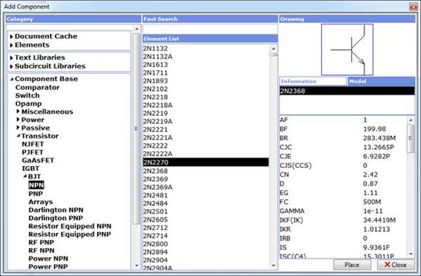
2. New Component Models
—
—
3. Graph Viewer
— A set of mathematical functions and expressions over state variables can be plotted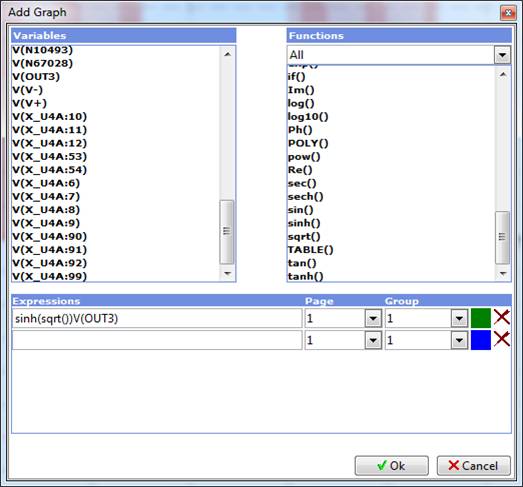
— Cursor functions are added
4. Schematic
— You can now create, modify and delete 
5. Modeling Management
— You can now easily work with simulations using
6. User Interface
"Graph" menu with following items is added:
— List
— Add Trace
— Cursor
— Data Points
— Export…
SimOne 1.1 Beta Changelog
Changes in Version 1.1.1
1. Simulations
— Speeding up simulation by not updating the status of latent devices is added. Simulation options are BYPASS, MBYPASS, BYTOL
— Damped Newton control options are added: sollim, sollimitev
— Following default simulation options were changed: DC_RELTOL =
— Initial approximation for DC Operating Point setting is available (NodeSet)
— Automatic step control in Transient Analysis and PSS Analysis is added
— In PSS Analysis plotting limits and step are not necessary now (default values refer to calculation limits)
2. Calculation Problems
— For better precision pivoting algorithm in
3. Schematic
— Simulation results display precision is 3 digits after the point
— Simulation results display on/off option is added
— Tolerance parameter for passive elements (R, L, C) is added
— Subcircuits with parametric inputs are added
— Mutual inductors can be used within subcircuits now
4. Fixed
— Dependent sources matrix parameters calculation
—
— Junction Gmin method in DC Operating Point
— PSS Analysis display
— Simulation relusts display for subcircuits
— SPICE netlist parcer
Changes in Version 1.1.0
1. Periodic Steady State Analysis (PSS Analysis)
Periodic behavior of the circuit is calculated using the Shooting Newton method while maintaining a
2. Schematic
— An option to display state variables in the last point of transient analysis or PSS result to the scheme is added
3. Modeling Management Module
— An interface for manual setting of state variables is added
— Initial conditions can now be set in different ways. In addition to operating point calculation and loading them from file, manual setting and zero initial conditions are available
— An automatic definition of maximal simulation threads amount is added. The threads amount choice depends on processing unit type
4. Results Display
— While not in multivariate analysis, resulting tables are vertically oriented which previously were horizontal
5. Fixed
— An ability to rename connection completely has been restored
— At Stability analysis tab "Show Eigenfrequencies Table" and "Show Eigenfrequencies Locus" checkboxes become available correctly
SimOne 1.0 Beta Changelog
Changes in Version 1.0.3
1. Multivariate Circuit Modeling
For each circuit analysis type, you can now perform:
— Temperature sweeps (.TEMP) — run the current calculations while varying the operating temperature
— Parameter sweeps (.PARAM) — run the current calculations while varying the parameters of schematic component models
2. Transient Analysis
— The algorithm for choosing the initial calculation step has been improved.
3. Stability Analysis
— You can now load the operating point from a file.
4. Schematic Elements
— Issues have been fixed in calculation of the parameters of the following models: diode, NJFET and PJFET field-effect transistors, GaAsFET transistor, NPN, PNP, NPN4 and PNP4 bipolar transistors
5. Schematic Editor
— You can move model names and element parameters around the schematic.
— You can edit element names and parameters without opening the parameter panel.
— The results of operating point calculations are displayed on the schematic.
6. Graphical Module
— The FastPlot graphical module’s new engine performs well when displaying large amounts of simulation data.
7. Implementation Specifics
— The new HDD access module lets you run simulations whose size is limited only by how much disk space is available.
— Multicore CPU architectures are supported better; this enables you to run multiple simulations at once without any performance hit and speed up versatile calculations. The maximum number of concurrent threads is configurable.
8.Data Export
— A number of simulation data export issues have been fixed.
Changes in Version 1.0.2
1. Simulation Control
— The Simulation Assistant has been introduced to help improve the use of data on typical schematic behaviors. The Simulation Assistant is available in Simulation. It is most useful when different analysis types need to be performed repeatedly while the structure of the schematic remains the same. In such situations, using the Simulation Assistant speeds up calculations; for large schematics, the speed gains can be tenfold and even hundredfold.
— A button has been added to the simulation options tab for resetting the default values for all parameters.
— Symbolic suffixes — such as m, p or n — can now be used for setting ranges in AC and Transient analysis options.
— The simulation storage format has been revised. Instead of a single .sim file, the simulation data is now split into multiple files:
.xml — Simulation parameters
.var — Information about the vectors of output variables
.dat — Simulation results
.cod — auxiliary information
2. Stability Analysis
— You can now select the algorithm for terminating the calculation of eigenvalues (EFCheckToITL) or zeroes in a Mihailov’s graph (CheckToITL).
3. Schematic Elements
— Issues have been fixed in parameter calculations for the PJFET, PNP and PNP4 transistor models.
— In the V-Switch and I-Switch models, a hysteretic switch mode (the VH, VT, IH and IT parameters) has been added. Issues have been fixed in uninterrupted mode calculations.
— A distortion-free Tline model has been added — The fading parameter of a Tline defines the damping of a signal in the line. A lossless line, which is a special case of this model, has a fading value of 1.
4. Data Export
— You can now export calculation results to the Excel, Matlab and Maple formats.
Changes in Version 1.0.1
1. Stability Analysis
— Multiple Mihailov hodograph representations have been introduced: in linear and normalized logarithmic scale.
— Issues have been fixed that affected calculations on low-order (order of 0 and 1) schematics and repeated launches of eigenvalue calculations.
2. DC Analysis
— The convergence of all operating point calculation methods has been improved.
— New parameters have been added to the DC analysis settings for better control of calculation method convergence.
— Issues have been fixed in the Source stepping, Gmin stepping and Junction Gmin stepping methods.
— The operating point can now be loaded from a text file.
3. Transient Analysis, AC Analysis
— The operating point can now be loaded from a text file.
4. Schematic Elements
— Models for NPN, PNP, NPN4 and PNP4 bipolar transistors have been added; the Gummel–Poon model is used.
5. Data Export
— You can now export calculation results as matrices and vectors in Matlab and Maple formats. This helps perform stability analysis independently in those systems.
6. Data Import in SPICE Format
— Issues have been fixed that affected export of voltage sources and bipolar transistors.
7. Document
— Simulations created for a .net document are now loaded the next time the document is opened, provided the document has been saved before it is opened.
8. User Interface
— A Help | About dialog box has been added.
— A menu item for the user manual has been added.
SimOne Electronic Circuit Analysis Program
SimOne provides the main types of circuit analysis common to SPICE modeling systems:
— DC analysis (.DC)
— AC analysis (.AC)
— Transient analysis (.TRAN)
— A new type: Stability analysis
The suite uses standard SPICE models of schematic components, such as:
— Resistor
— Capacitor
— Inductor
— Transformer
— Tline
— Waveform and dependent current and voltage sources
— Controlled switches
— Diode
— NJFET and PJFET junction field-effect transistors (Shichman–Hodges model)
— GaAsFET gallium arsenide field-effect transistors
— LEVEL = 1–5
— NPN and PNP bipolar transistors (Gummel–Poon model)